Motivation for RNA-Seq quantification
Typical studies:
DNA-Seq -> alignment -> variant calling -> genome wide association study (GWAS);
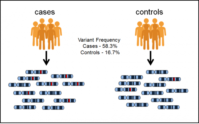
RNA-Seq -> alignment -> quantification -> differential expression analysis
RNA-Seq quantification
Counting versus probabilistic estimation dilemma is (mostly) about doing analysis on gene versus transcript level.
- When quantifying on gene level - we simply count the number of reads aligned to each gene.
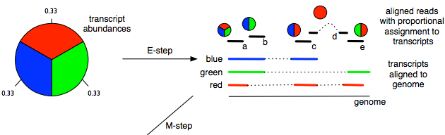
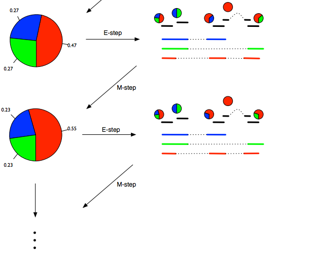
- On transcript level, we need an algorithm such as the Expectation Maximization (EM, pictured below) to deal with the uncertainty.
When performing statistical analysis of RNA expression, doing it on gene level compared to transcript level is more robust and experimentally actionable. The biologists will also usually draw their conclusions on gene level since that's the level that the biological pathways are annotated on.
However, the use of gene counts for statistical analysis can mask transcript-level dynamics. A popular alternative nowadays is to estimate the transcript abundances and then aggregate to gene level, or perform the entire analysis on trancsript level (testing for differential expression) and then aggregate the results.
Gene level quantification
We shall, for simplicity's sake, only perform gene level quantification. Even though it has some drawbacks, it's a strategy still used by most genomic scientists. Here's what we have at the beginning of the quantification step and what we want to estimate:
- We have: aligned reads and annotations. A file format called SAM/BAM is now the standard formats for next-generation sequence alignments.
- We estimate: relative abundance.
We'll start with some simple methods to find if two intervals overlap.
def overlap(x, y):
    """
    This function takes two intervals and determines whether
    they have any overlapping segments.
    """
    new_start = max(x[1], y[1])
    new_end = min(x[2], y[2])

    if new_start < new_end and x[0] == y[0]:
        return True
    return False
We will define four intervals as tuples.
region1 = ("chr3", 27, 82)
region2 = ("chr4", 27, 82)
region3 = ("chr3", 57, 75)
overlap(region1, region2)
overlap(region1, region3)
We shall now pick a gene of interest and try to find reads mapping to that gene.
# the location of DEFB125 gene in human genome, gencode.v27 annotation
gene = ('chr20', 87249, 97094)
To start exploring reads from a SAM/BAM file, we first need to load the file.
import pysam

# load BAM file
bamfile = pysam.AlignmentFile("aligned/sample_01_accepted_hits.bam", "rb")
Note the 'rb' parameter indicates to read the file as binary, which is the BAM format (BAM stands for Binary Alignment Map). If loading a SAM file, this parameter does not need to be specified.
An important and very common application is to count the number of reads (aligned fragments) that overlap a given feature (i.e. region of the genome or gene). One simple approach to doing this is to make a list of all reads generated and simply iterate over the reads to identify whether a read overlaps a region.
In this case we need an overlap method that can compare a simple interval (defined by a tuple of sequence, start, end) with a pysam AlignedSegment object. This overlap method also needs the AlignmentFile object to decode the chromosome name.
def overlap(x, gene, bamfile):
    """
    A modified version of overlap that takes an interval and a pysam
    AlignedSegment and tests for overlap
    """
    new_start = max(x.reference_start, gene[1])
    new_end = min(x.reference_end, gene[2])

    if (new_start < new_end and bamfile.getrname(x.tid) == gene[0]):
        return True

    return False
%%time

# code to iterate over reads and count for a single gene
naive_gene_count = 0

for x in bamfile.fetch():
    # Note x is of type pysam.AlignedSegment
    if(overlap(x, gene, bamfile)):
        naive_gene_count += 1
print(naive_gene_count)
The problem with this approach is that to do this, you will need to store the entire file in memory. Worse than that, in order to find the reads within a single gene, you would need to iterate over the entire file, which can contain hundreds of millions of reads. This is quite slow even for a single gene, but will only increase if you want to look at many genes.
Instead, more efficient datastructures (and indexing schemes) can be used to retrieve reads based on positions in more efficient ways.
To get the reads overlapping a given region, Pysam has a method called fetch(), which takes the genomic coordinates and returns an iterator of all reads overlapping that region.
bam_iter = bamfile.fetch(gene[0], gene[1], gene[2])
%%time

pysam_gene_count = 0

for x in bam_iter:
    pysam_gene_count += 1
print(pysam_gene_count)
Not surprisingly, they are the same - the big difference is that the second method is significantly faster. The reason for this is that Pysam (like Samtools, Picard, and other similar toolkits) make use of clever tricks to index the file by genomic positions to more efficiently search for reads within a given genomic interval.
Now that we know how to count reads overlapping a region, we can write this as a function and try and compute this for all genes.
def read_count(gene, bamfile):
    """
    Compute the number of reads contained in a bamfile that overlap
    a given interval
    """
    bam_iter = bamfile.fetch(gene[0], gene[1], gene[2])

    pysam_gene_count = 0

    for x in bam_iter:
        pysam_gene_count += 1

    return pysam_gene_count
You can run this with any gene tuple now:
# the location of ZNFX1 gene in human genome, gencode.v27 annotation
gene2 = ("chr20", 49237945, 49278426)

read_count(gene2, bamfile)
Now, let's compute the gene counts for all genes. We'll start by reading in all genes:
%%time

gene_counts={}

with open('gencode.v27.chr20.bed', 'r') as f:
    for line in f:
        tokens = line.split('\t')
        gene_local = (tokens[0], int(tokens[1]), int(tokens[2]))
        count = read_count(gene_local, bamfile)
        gene_counts.update({tokens[3].rstrip() : count})
Now it's easy to query the gene counts for different genes.
print(gene_counts.get("ARFGEF2"))
print(gene_counts.get("SOX12"))
print(gene_counts.get("WFDC8"))
(Within-sample) Normalization
In previous slides, we've seen how we can compute raw counts, i.e. number of reads that align to a particular feature (gene or transcript).
$$X_{i}$$
These numbers are heavily dependent on two things:
- The amount of fragments sequenced
- The length of the feature, or more appropriately, the effective length. Effective length refers to the number of possible start sites a feature could have generated a fragment of that particular length. In practice, the effective length is usually computed as:
$$\widetilde{l_{i}}=l_{i}-\mu_{FLD}+1$$
Since counts are NOT scaled by the length of the feature, all units in this category are not comparable within a sample without adjusting for the feature length!
Different units
- Reads Per Kilobase per Million reads mapped (RPKM), or for the paired-end reads: FPKM (Fragments instead of Reads).
$$FPKM_{i}=\frac{X_i}{\left ( \frac{\widetilde{l_{i}}}{10^{3}}\left ( \frac{N}{10^{6}} \right ) \right )} = \frac{X_i}{\widetilde{l_{i}}N}\cdot 10^{9}$$
- Transcripts Per Million (TPM)
$$TPM_{i}=\frac{X_i}{\widetilde{l_{i}}}\cdot \left ( \frac{1}{\Sigma_{j}\frac{X_j}{\widetilde{l_{j}}}} \right ) \cdot 10^{6}$$
import pandas as pd

counts = {'Gene Name': ['A(2kb)', 'B(4kb)', 'C(1kb)', 'D(10kb)'],
          'Rep1 Counts': [10, 20, 5, 0],
          'Rep2 Counts': [12, 25, 8, 0],
          'Rep3 Counts': [30, 60, 15, 1]
         }

df = pd.DataFrame(counts, columns= ['Gene Name', 'Rep1 Counts', 'Rep2 Counts', 'Rep3 Counts']).set_index('Gene Name')

df
Let's first calculate the abundances in FPKM units. We first divide by the total number of reads:
# library size normalization (division by 10 instead of 10^6)
df_rpkm = df.div(df.sum()/10).round(2)
df_rpkm
Then we normalize for gene length:
# save gene sizes in new column
df_rpkm['kb'] = [2,4,1,10]

# gene size normalization
df_rpkm = df_rpkm.div(df_rpkm.kb, axis=0).round(2)
df_rpkm.drop(['kb'], axis=1)
The sums of total normalized counts in each column are not equal as we prove below:
# FPKM normalization sums per samples are not equal (samples are not comparable).
df_rpkm.drop(['kb'], axis=1).sum()
Now we will calculate the abundances in TPM units. Here, the first thing we do is normalize for gene length!
df_tpm = df
# save gene sizes in new column
df_tpm['kb'] = [2,4,1,10]

# gene size normalization is performed first
df_tpm = df_tpm.div(df_tpm.kb, axis=0).round(2)
df_tpm.drop(['kb'], axis=1)
And now we perform the library size normalization, using abundances already normalized for gene length:
# library size normalization (division by 10 instead of 10^6)
df_tpm = df_tpm.div(df_tpm.sum()/10).round(3)
df_tpm.drop(['kb'], axis=1)
The sums of total normalized counts in each column are now equal (when using TPM)!
# TPM normalization sums per samples are equal (samples are comparable).
df_tpm.drop(['kb'], axis=1).sum()
def tpm(genefile, bamfile):
    """
    Compute the TPM (transcripts per million) metric for all genes within the genefile using
    an RNA-Seq bamfile
    """
    total_mapped_reads = 0

    # here you want all reads
    bam_iter = bamfile.fetch()

    for x in bam_iter:
        total_mapped_reads += 1

    gene_counts = {}
    with open(genefile, 'r') as f:
        for line in f:
            tokens = line.split('\t')
            gene_local = (tokens[0], int(tokens[1]), int(tokens[2]))
            gene_length = gene_local[2] - gene_local[1]
            raw_count = read_count(gene_local, bamfile)
            if tokens[3] in gene_counts:
                gene_counts[tokens[3]] = (gene_counts[tokens[3]][0] + raw_count, gene_length)
            else:
                gene_counts.update({tokens[3].rstrip() : (raw_count, gene_length)})

    countsDF = pd.DataFrame(gene_counts, index=['raw_count', 'gene_length'])
    countsDF = countsDF.T
    X=countsDF.iloc[:,0].values
    l=countsDF.iloc[:,1].values
    countsDF = countsDF.assign(tpm = 1e6 * (X/l) / (X/l).sum())
    return(countsDF)
%%time

gene_counts = tpm('gencode.v27.chr20.bed', bamfile)
gene_counts.head(10)
def rpkm(genefile, bamfile):
    """
    Compute the RPKM (reads per kilobase per million mapped reads) metric for all genes within the genefile using
    an RNA-Seq bamfile
    """
    total_mapped_reads = 0

    # here you want all reads
    bam_iter = bamfile.fetch()

    for x in bam_iter:
        total_mapped_reads += 1

    gene_counts = {}
    with open(genefile, 'r') as f:
        for line in f:
            tokens = line.split('\t')
            gene_local = (tokens[0], int(tokens[1]), int(tokens[2]))
            gene_length=gene_local[2]-gene_local[1]
            raw_count = read_count(gene_local, bamfile)
            rpk_metric = 1e9 * raw_count \
                            / (total_mapped_reads * gene_length)
            gene_counts.update({tokens[3].rstrip() : (raw_count, gene_length, rpk_metric)})

    countsDF = pd.DataFrame(gene_counts, index=['raw_count', 'gene_length', 'rpkm'])
    countsDF = countsDF.T
    return(countsDF)
%%time

gene_counts_rpkm = rpkm('gencode.v27.chr20.bed', bamfile)
gene_counts_rpkm.head(10)